Introduction
Hello there, Workout Wednesday #DataFam! This week’s challenge is all about two of my passions growing up: baseball and physics. This past baseball season, New York Yankees outfielder Aaron Judge broke the 61 year old American League record for home runs in a single season set by Roger Maris in 1961 – Judge concluded the 2022 regular season with 62 home runs.
Several months ago, I stumbled across a Twitter profile (@would_it_dong) built by Dan Morse that uses Baseball Savant/MLB StatCast hit measurement data to approximate whether a hit would be a home run in each of the 30 MLB ballparks. I was curious if I could model hit trajectory data using Tableau. Could I take simple numeric inputs (launch angle and exit Velocity) and build out a tool that would display the trajectory of a batted ball over time until it lands. Reflecting on my childhood fascination with how things move (physics), I researched the relevant equations and developed this dashboard.
The challenge this week is straightforward, but challenging. Using the equations I have provided, use data densification, table calculations, and pages to model Aaron Judge’s home run trajectories with Tableau! Also be sure to cite Baseball Savant and Statcast for the data and Goodware via Flaticon for the baseball icon.
I will be sharing a solution video later this week, so if you can’t figure it out by then, stay tuned and I’ll show you how I did it!
Enjoy the workout!
Requirements
- Dashboard Size: 1250 x 1000px
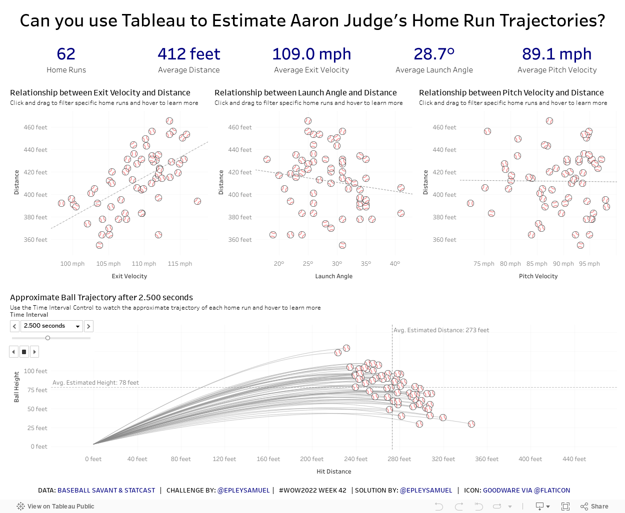
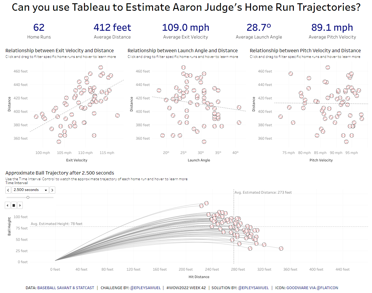
- 5 sheets (1 KPI, 3 Scatterplot, 1 Trajectory Plot)
- Match KPIs (Value Font: 24, #000080; Label Font: 11, #000000)
- Create three scatterplots with filter actions that apply to the KPIs and the hit trajectory model, but not the other scatterplots. When hits are filtered in one scatterplot, create a highlight action to show the selected hits in the other two scatterplots. Also, include a regression line in each scatterplot.
- Exit Velocity (mph) vs Distance (feet)
- Launch angle (degrees) vs Distance (feet)
- Pitch Velocity (mph) vs Distance (feet)
- Create a Ball Trajectory Plot, with Hit Distance on the X-axis (fixed from -39 feet to 479 feet) and Ball Height on the Y-axis (fixed from -5 feet to 160 feet)
- Show the Position of the ball at the start of each time stamp. When modeling the Y-axis, ensure that all values are at or above zero. When modeling the X-axis, once the Ending Y Position is at or below zero, have the Ending X Position values stop as well.
- Leverage the pages card with the time interval and show history, with Trails only for all points (50% transparency, #898989, smallest line)
- See Ball Trajectory Formulas below for the physics formulas required to calculate the trajectory (you’ll turn these into Tableau Calculations)
- Match tooltips, formatting, labels, and reference lines
Bonus:
- You can add the custom shapes of the baseballs (available on Data.World) to the Shapes file within your ‘My Tableau Repository’ folder. Here’s a tutorial by Carly Capitula from Interworks about how to load your own custom shapes!
- For each point on the scatterplots, create a way to rotate each of the balls so they are randomly pointing in one of nine different orientations.
- For each point on the ball trajectory plot, make it look like the ball is rotating counter-clockwise as the page plays.
Dataset
This week uses a custom data set. You can find it here on Data.World
Ball Trajectory Formulas
- Given how complicated physics can be for some folks, I wanted to provide you with as many tips and pointers when you are wrestling with this challenge. There are a few helpful things to remember when working in physics:
- Position is the location of an object at a specific point in time. Units for Position are often referred to in m, or meters.
- Velocity is the rate of change of an object’s Position over an amount of difference in time (our time-step for this challenge is 0.025 seconds). In calculus terms, Velocity is the “derivative” of Position. Units for Velocity are often referred to in m/s, or meters per second.
- Acceleration is the rate of change of an object’s Velocity (the derivative of Velocity, or the second-order derivative of Position). Units for acceleration are often referred to in m/s^2, or meters per second squared.
- Constants (consider using parameters for each of these)
- Baseball Mass: 0.145 kg
- Cross Sectional Area: 0.00426 m^2
- Drag Coefficient: 0.4
- Gravity: -9.81 m/s^2
- Y Position Start: 1.0 m
- Time Interval: 0.025 seconds
- Conversion of mph to m/s: divide mph by 2.237 to get m/s
- Conversion of m/s to mph: multiply m/s by 2.237 to get mph
- Conversion of meters to feet: multiply meters by 3.28084 to get feet
- Conversion of feet to meters: divide feet by 3.28084 to get meters
- The general order you will want to think about these equations is as follows:
- Start: Starting Position and Starting Velocity.
- Change: Force (drag/air resistance and gravity) changes Velocity (acceleration/deceleration) resulting in Ending Velocity. This change in Velocity allows us to determine the change in Position at a certain moment in time.
- End: Ending Position is determined by taking the Starting Position plus Ending Velocity multiplied by the amount of time that has elapsed.
- Ending Position = Starting Position + (Ending Velocity * 0.025)
- Position:
- The unit of measure we want to use for Position calculations is in meters. There shouldn’t be any conversions needed at the start, but since the final output shows distances and heights in feet, you will need to convert when it’s all said and done.
- The Starting Position of the ball at [Time Interval] = 0 will be X = 0.0m, Y = 1.0m. We’re going to assume that Aaron Judge hit the ball at about waist height. At each time step, you should have a Starting Position and an Ending Position.
- The Starting Position should equal the Ending Position of the previous step.
- As mentioned earlier, the Ending Position is calculated from taking the Starting Position and figuring out how much distance was covered over a specific amount of time (the time interval of 0.025 seconds).
- Velocity:
- The unit of measure we want to use for Velocity is in meters per second, so you will need to change miles per hour into meters per second using the conversion factor mentioned above. Note that Estimated Velocity (in the tooltip) is in miles per hour, so you will have to convert this back.
- The initial Velocity of the ball (at Time Interval = 0) is aimed at a specific Launch Angle. Using trigonometry, we can break this Velocity into its respective X and Y components:
- For X (horizontal), use the following to determine the Initial Velocity: Exit Velocity * COS(RADIANS( Launch Angle ))
- For Y (vertical), use the following to determine the Initial Velocity: Exit Velocity * SIN(RADIANS(Launch Angle))
- At each time step, the ball starts at a specific Velocity. In the horizontal direction (X), the only force acting on the ball after it is hit is drag. In the vertical direction (Y), there are two forces acting on the ball: gravity and drag (see the acceleration section for more details).
- The Estimated Velocity in the tooltip can be calculated using the Pythagorean Theorem. Imagine a right triangle where the two known sides are the Ending X Velocity and Ending Y Velocity and the hypotenuse is the Estimated Velocity.
- Similar to how the Ending Position is calculated by taking the Starting Position and the End Velocity times a time step, Ending Velocity is calculated by taking Starting Velocity and adding the Force times a time step. Since Force = Mass * Acceleration, we have to divide the Force by the Mass of the baseball in order to calculate the Acceleration of the ball at that moment. So, in formula form it would looks something like this:
- Ending Velocity = Starting Velocity + (Force / Mass * 0.025)
- Acceleration:
- There will be two forces acting on the ball at any given point in time: Drag (also known as Air Resistance) and Gravity.
- Drag is the interaction of a solid body with a fluid (liquid or gas). Basically, it is a force that slows down a baseball’s Velocity. The formula for Drag is as follows:
- -0.5* Drag Coefficient * Air Density * Cross Sectional Area * Starting Velocity ^2
- Gravity is a constant force that is pulling objects toward the Earth’s surface. The formula for Gravity Force is as follows:
- Baseball Mass * Gravity Acceleration
- Hints for the calculation logic:
- If you exclusively use the LOOKUP() function, you may encounter circular reference errors. Consider how LOOKUP is similar to PREVIOUS_VALUE.
- A few caveats to hopefully satisfy the “gotchas” that might be brought up by any physics experts out there:
- Remember that each component of projectile motion takes place along both a horizontal (X) and vertical (Y) axis. You will need to break these out in order to properly calculate them.
- Baseball Savant only provides us with the Launch Angle and the Exit Velocity. This means that our projectile motion equations will not allow us to easily account for angular rotation which could impact the flight of the ball. This type of force is what’s known as the Magnus Effect. Also, for the simplicity of the modeling, we are going to avoid attempting to calculate the Coriolis Effect or the effect on the movement of the ball due to the earth’s rotation.
- To ensure that the estimate is as close to the Baseball Savant reported distance, I adjusted the Air Density for each home run. In reality, air density doesn’t vary as much as [Air Density Estimate] would suggest, but this was the easiest way to control for factors that we cannot model.
Attribute
When you publish your solution on Tableau Public make sure to take the time and include a link to the original inspiration. Also include the hashtag #WOW2022 in your description to make it searchable!

Share
After you finish your workout, share on Twitter using the hashtag #WOW2022 and tag @EpleySamuel, @LukeStanke, @_Lorna_Brown, @HipsterVizNinja, @_hughej, and @YetterDataViz
Solution
Interactive